0%

vanishing gradients

Vanishing Gradients

这里只使用numpy来实现一个neural network,而非借助pytorch这样的框架,如此,可以更好的帮助我理解neural network以及vanishing gradients.

1
2
3
4
5
6
7
8
9
10
import numpy as np
import matplotlib.pyplot as plt

%matplotlib inline
plt.rcParams['figure.figsize'] = (10.0, 8.0) # set default size of plots
plt.rcParams['image.interpolation'] = 'nearest'
plt.rcParams['image.cmap'] = 'gray'

%load_ext autoreload
%autoreload 2
1
2
3
4
5
6
7
8
9
10
11
12
13
14
15
16
17
18
# generate random data -- not linearly separable
np.random.seed(0)
N = 100 # number of points per class
D = 2 # dimensionality (向量维度)
K = 3 # number of classes
X = np.zeros((N*K, D))
num_train_examples = X.shape[0]
y = np.zeros(N*K, dtype='uint8') # 无符号整数
for j in range(K):
ix = range(N*j, N*(j+1))
r = np.linspace(0.0, 1, N) # radius, evenly spaced numbers
t = np.linspace(j*4, (j+1)*4, N) + np.random.randn(N)*0.2 # theta
X[ix] = np.c_[r*np.sin(t), r*np.cos(t)] # 变成2列的matrix
y[ix] = j
fig = plt.figure()
plt.scatter(X[:,0], X[:,1], c=y, s=40, cmap=plt.cm.Spectral)
plt.xlim([-1,1])
plt.ylim([-1,1])

svg

sigmoid 函数的值在0,1之间,尤其是在输入值的绝对值很大的情况下,两端会无限接近0或1,因此变得很扁平,由此,对应的梯度(Gradient)就会无限逼近0。这就导致了所谓的梯度消失(vanishing gradients)的现象。因为梯度消失使得神经网络无法进行有效的学习(因为每次迭代对参数W的修正几乎都是0)。

而另一方面,relu函数不会出现因为输入参数变大而输出变得不敏感。

1
2
3
4
5
6
7
8
9
def sigmoid(x):
x = 1/(1+np.exp(-x))
return x

def sigmoid_grad(x): # sigmoid函数的导数
return (x)*(1-x)

def relu(x):
return np.maximum(0,x)
1
2
3
4
5
6
# plot the 2 function
x = np.linspace(-3,3,100)
y_sigmoid = sigmoid(x)
y_relu = relu(x)

plt.plot(x, y_sigmoid, 'b-', x, y_relu, 'r-')

svg

接下来让我们看一下2种不同的非线性函数(sigmoid和relu)对神经网络在训练时的影响。以下,我们会创建一个简单的3层神经网路(2 hidden layers)。 通过使用sigmoid和relu我们可以比较在训练过程中的区别。

1
2
3
4
5
6
7
8
9
10
11
12
13
14
15
16
17
18
19
20
21
22
23
24
25
26
27
28
29
30
31
32
33
34
35
36
37
38
39
40
41
42
43
44
45
46
47
48
49
50
51
52
53
54
55
56
57
58
59
60
61
62
63
64
65
66
67
68
69
70
71
72
73
74
75
76
77
78
79
80
81
82
83
84
85
86
87
88
89
90
91
92
93
94
95
96
97
98
99
100
101
102
103
104
105
106
107
108
109
110
111
112
113
114
115
116
117
# function to train a 3 layer neural net with either relu or sigmoid nonlinearity via vanilla grad decent.
def three_layer_net(NONLINEARITY, X, y, model, step_size, reg):
# param init
h = model['h']
h2 = model['h2']
W1 = model['W1']
W2 = model['W2']
W3 = model['W3']
b1 = model['b1']
b2 = model['b2']
b3 = model['b3']

# some hyperparameters

# gradient descent loop
num_examples = X.shape[0]
plot_array_1 = []
plot_array_2 = []
for i in range(50000):
# forward prop
# 假设有X的维度[N, M], 即有N条training 数据,每条数据有M个feature
if NONLINEARITY == 'RELU':
# 从X到hidden layer 1, X=[N*2], W1=[2*50] --> hidden layer=[N*50]
hidden_layer = relu(np.dot(X,W1) + b1)
# 从 hidden layer 1 到 layer2. hidden 1 = [N*50], W2=[50*50]-->hidden2 = [N*50]
hidden_layer2 = relu(np.dot(hidden_layer, W2) + b2)
# 从 hidden 2 到 最总output layer, hidden 2 = [1*50], W3=[50*3] --> output = [3]
scores = np.dot(hidden_layer2, W3) + b3 # scores的维度是[N,3]

elif NONLINEARITY == 'SIGM':
hidden_layer = sigmoid(np.dot(X,W1) + b1) # 从X到hidden layer 1
hidden_layer2 = sigmoid(np.dot(hidden_layer, W2) + b2) # 从 hidden layer 1 到 layer2
scores = np.dot(hidden_layer2, W3) + b3

exp_scores = np.exp(scores) # [N*K], K=3
# keepdims=True 意思是np.sum被sum的维度变为1,另一个维度保持不变。
probs = exp_scores / np.sum(exp_scores, axis=1, keepdims=True) # normalize,行方向sum

# compute the loss: average cross-entropy loss and regularization
corect_logprobs = -np.log(probs[range(num_examples), y]) # y的取值范围0,1,2。结果[N*1]
data_loss = np.sum(corect_logprobs)/num_examples
# regularization项
reg_loss = 0.5*reg*np.sum(W1*W1) + 0.5*reg*np.sum(W2*W2)+0.5*reg*np.sum(W3*W3)
loss = data_loss + reg_loss
# if i % 1000 == 0:
# print("iteration {0}: loss {1}".format(i, loss))

# comput the gradient on scores
dscores = probs # -- [N*K]
dscores[range(num_examples), y] -= 1 # error value -- [N*K]
dscores /= num_examples

# backprop here
# 从output layer back prop 到 hidden layer2, 由于该层没有nonlinearity
# 即 hidden2*W3 = s, ds/dW3 = hidden2 (local gradient), 因此back prop error
# 只需要将error * local gradient,即hidden2.
dW3 = (hidden_layer2.T).dot(dscores) # [50*N] * [N*3] = [50*3]
db3 = np.sum(dscores, axis=0, keepdims=True) # [3]

if NONLINEARITY == 'RELU':
# backprop Relu nonlinearity here
dhidden2 = np.dot(dscores, W3.T)
dhidden2[hidden_layer2 <= 0] = 0
dW2 = np.dot(hidden_layer.T, dhidden2)
plot_array_2.append(np.sum(np.abs(dW2))/np.sum(np.abs(dW2.shape)))
db2 = np.sum(dhidden2, axis=0)
dhidden = np.dot(dhidden2, W2.T)
dhidden[hidden_layer <= 0] = 0

elif NONLINEARITY == 'SIGM':
# backprop sigmoid nonlinearity there
# hidden layer 2 是 sigmoid的输出,因此需要乘以一个local gradiant
dhidden2 = dscores.dot(W3.T)*sigmoid_grad(hidden_layer2)
dW2 = (hidden_layer.T).dot(dhidden2)
plot_array_2.append(np.sum(np.abs(dW2))/np.sum(np.abs(dW2.shape)))
db2 = np.sum(dhidden2, axis=0)
dhidden = dhidden2.dot(W2.T)*sigmoid_grad(hidden_layer)

dW1 = np.dot(X.T, dhidden)
plot_array_1.append(np.sum(np.abs(dW1))/np.sum(np.abs(dW1.shape)))
db1 = np.sum(dhidden, axis=0)

# add regularization
dW3 += reg * W3
dW2 += reg * W2
dW1 += reg * W1

# option to return loss, grads,
# grads = {}
# grads['W1'] = dW1
# grads['W2'] = dW2
# grads['W3'] = dW3
# grads['b1'] = db1
# grads['b2'] = db2
# grads['b3'] = db3

# update grads
W1 += -step_size * dW1
b1 += -step_size * db1
W2 += -step_size * dW2
b2 += -step_size * db2
W3 += -step_size * dW3
b3 += -step_size * db3
# evaluate training set accuracy, 使用training出来的W1,W2,W3,b1,b2,b3
# 来计算结果。
if NONLINEARITY == 'RELU':
hidden_layer = relu(np.dot(X, W1) + b1)
hidden_layer2 = relu(np.dot(hidden_layer, W2) + b2)
elif NONLINEARITY == 'SIGM':
hidden_layer = sigmoid(np.dot(X, W1) + b1)
hidden_layer2 = sigmoid(np.dot(hidden_layer, W2) + b2)

scores = np.dot(hidden_layer2, W3) + b3
predicted_class = np.argmax(scores, axis=1) # 找出每一行的最大值的index
print('training accuracy: {0}'.format(np.mean(predicted_class==y)))

return plot_array_1, plot_array_2, W1, W2, W3, b1, b2, b3

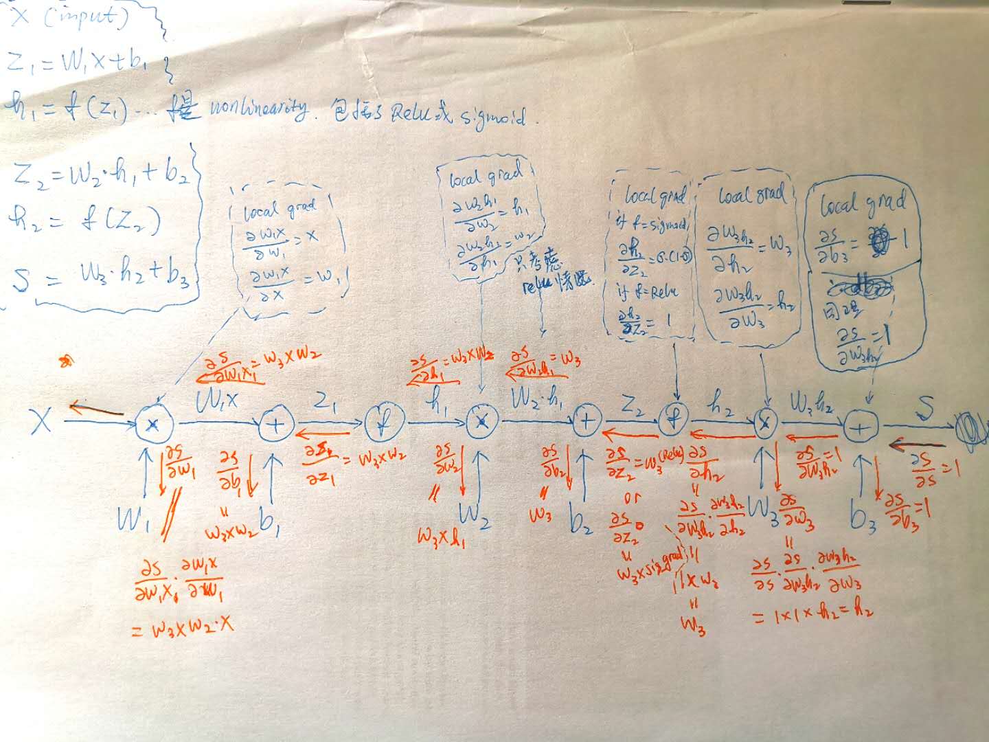
关于back propagation 的计算参见下图。 其实就是对chain rule的应用。

Train net with sigmoid nonlinearity first

1
2
3
4
5
6
7
8
9
10
11
12
13
14
15
16
17
18
19
20
# Initialize toy model, train sigmoid net 

N = 100 # number of points per class
D = 2 # dimensionality
K = 3 # number of classes
h = 50 # hidden layer 1 size
h2 = 50 # hidden layer 2 size
num_train_examples = X.shape[0]

model = {}
model['h'] = h
model['h2'] = h2
model['W1'] = 0.1 * np.random.randn(D, h)
model['b1'] = np.zeros((1,h))
model['W2'] = 0.1 * np.random.randn(h, h2)
model['b2'] = np.zeros((1,h2))
model['W3'] = 0.1 * np.random.randn(h2, K)
model['b3'] = np.zeros((1,K))

(sigm_array_1, sigm_array_2, s_W1, s_W2, s_W3, s_b1, s_b2, s_b3) = three_layer_net('SIGM', X, y, model, step_size=1e-1, reg=1e-3)

training accuracy: 0.97

Now train net with ReLU nonlinearity

1
2
3
4
5
6
7
8
9
10
11
12
# Re-initialize model, train relu net
model = {}
model['h'] = h
model['h2'] = h2
model['W1'] = 0.1 * np.random.randn(D, h)
model['b1'] = np.zeros((1,h))
model['W2'] = 0.1 * np.random.randn(h, h2)
model['b2'] = np.zeros((1,h2))
model['W3'] = 0.1 * np.random.randn(h2, K)
model['b3'] = np.zeros((1,K))

(relu_array_1, relu_array_2, r_W1, r_W2, r_W3, r_b1, r_b2, r_b3) = three_layer_net('RELU', X, y, model, step_size=1e-1, reg=1e-3)

training accuracy: 0.9933333333333333

The Vanishing Gradient Issue — 梯度消失的问题

我们可以对某一hidden层W的梯度(dW)进行加总,用这个简单的指标来衡量学习的速度,显然,sum(dW)越大,说明神经网络的学习速度越快。

1
2
3
4
plt.plot(np.array(sigm_array_1))
plt.plot(np.array(sigm_array_2))
plt.title('Sum of magnitudes of gradients -- SIGM weights')
plt.legend(("sigm first layer", "sigm second layer"))

svg

由上图可见,第二层的梯度显著大于第一层。说明在进行back prop的时候,hidden层越多,那么排在最前的hidden层对应的梯度(dW)就会变得越来越小。直观的讲,因为chain rule的原因,hidden层越多,则chain rule里乘的local gradient越多,而另一方面,由于nonlinearity使用的是sigmod,sigmoid grad = δ*(1-δ),输出必在[0,1]之间。所以local gradient的值都落在[0,1],那么随着hidden层的增加,排在最前的hidden层对应的梯度(dW)就会变得越来越小。

1
2
3
4
plt.plot(np.array(relu_array_1))
plt.plot(np.array(relu_array_2))
plt.title('Sum of magnitudes of gradients -- ReLU weights')
plt.legend(("relu first layer", "relu second layer"))

svg

由上图可见,ReLU收敛的速度比sigmoid快很多,而且收敛后就很稳定。

1
2
3
4
5
6
7
# overlaying the 2 plots to compare
plt.plot(np.array(sigm_array_1))
plt.plot(np.array(sigm_array_2))
plt.plot(np.array(relu_array_1))
plt.plot(np.array(relu_array_2))
plt.title('Sum of magnitudes of gradients -- hidden layer neurons')
plt.legend(("sigm first layer", "sigm second layer", "relu first layer", "relu second layer"))

svg

上图可以更明显的看到,ReLU的收敛速度快,一开始的gradient更高。

最后,看看2种分类器的表现,由于ReLU训练速度更快,因此用同样的epochs,ReLU表现的更好。

1
2
3
4
5
6
7
8
9
10
11
12
13
14
# plot the classifiers -- SIGMOID
h = 0.02
x_min, x_max = X[:, 0].min() - 1, X[:, 0].max() + 1
y_min, y_max = X[:, 1].min() - 1, X[:, 1].max() + 1
xx, yy = np.meshgrid(np.arange(x_min, x_max, h),
np.arange(y_min, y_max, h))
Z = np.dot(sigmoid(np.dot(sigmoid(np.dot(np.c_[xx.ravel(), yy.ravel()], s_W1) + s_b1), s_W2) + s_b2), s_W3) + s_b3
Z = np.argmax(Z, axis=1)
Z = Z.reshape(xx.shape)
fig = plt.figure()
plt.contourf(xx, yy, Z, cmap=plt.cm.Spectral, alpha=0.8)
plt.scatter(X[:, 0], X[:, 1], c=y, s=40, cmap=plt.cm.Spectral)
plt.xlim(xx.min(), xx.max())
plt.ylim(yy.min(), yy.max())

svg

1
2
3
4
5
6
7
8
9
10
11
12
13
14
# plot the classifiers-- RELU
h = 0.02
x_min, x_max = X[:, 0].min() - 1, X[:, 0].max() + 1
y_min, y_max = X[:, 1].min() - 1, X[:, 1].max() + 1
xx, yy = np.meshgrid(np.arange(x_min, x_max, h),
np.arange(y_min, y_max, h))
Z = np.dot(relu(np.dot(relu(np.dot(np.c_[xx.ravel(), yy.ravel()], r_W1) + r_b1), r_W2) + r_b2), r_W3) + r_b3
Z = np.argmax(Z, axis=1)
Z = Z.reshape(xx.shape)
fig = plt.figure()
plt.contourf(xx, yy, Z, cmap=plt.cm.Spectral, alpha=0.8)
plt.scatter(X[:, 0], X[:, 1], c=y, s=40, cmap=plt.cm.Spectral)
plt.xlim(xx.min(), xx.max())
plt.ylim(yy.min(), yy.max())

svg

欢迎关注我的其它发布渠道